Dating Isn’t Really That Hard!

My darling bride’s definition of “a first date” was getting dressed up and having a lousy time. That is, until she met… your humble servant…

As it sometimes happens, “Date”-ing in Excel can sometimes yield a lousy presentation, but it doesn’t have to be so. If you get it done correctly, it becomes a breeze. Let’s take a look at how to make “Date”-ing easy in Excel.

Before we get started….

Here are a couple of “Save Your Life” tips regarding dates. There are two keyboard combinations that could save you some time. Also, for the purposes of this posting, the formulae will refer to either “TheDate” or “TheDateText” as listed below.

The Parts of a Date

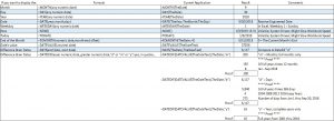
Excel has a few functions that allow you to parse the elements of a date. Note that the date as presented in the spreadsheet is a FORMATTING issue as typically, the dates are stored as numbers. As numbers, you can add days to the date or subtract one date from another. There is even a way to convert a text date (string) into a numeric date with just a formula!

Below, you’ll find a table with some of the date related formulae I’ve found to be most useful. The table lists formulae to parse out the elements of a date as well as finding the number of days, months or years between two dates. You’ll also find the formula to convert date text strings into a number (This is definitely a “Save Your Life” tip especially if you use downloaded data!)

Putting Dynamic Dates in Text Strings

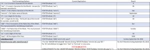
Now that we know that the date is a number, how do we incorporate the dates into text strings? The formula I’ve found to be most useful in this situation is “=TEXT()” (sans quotes). You can nest the =TEXT() formula within other formulae to achieve the presentation you desire.

The syntax for the formula is:

=Text(any numeric date, “date format”)

And, yes, you’ll need the double quotes.

The table below provides the basic building blocks for using the =TEXT() formula.

Dates With Custom Formats

There are custom formats that you can apply to the dates to circumvent the use of the “=TEXT()” formula.

Custom Formats can simplify and stabilize presentations.

A possible drawback to “text” formatting is that it might require a “helper” cell or reference. In other words, the “=Text()” formula might require a reference to another cell or data point that contains the date.

To resolve the drawback, you can use a “Custom” format. If the cell contains a custom format, a “helper” cell is not required. Simply input the date in the presentation cell and the custom formatting will present the date according the custom format you’ve created.

For example, if you wanted to ensure that the date presentation for your company’s quarterly Income Statement is always correct, you’ll need to create a custom format via the Format Cells dialogue box.

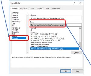
To create the custom formatting, right mouse click and open the Formatting Cells Dialogue box.

In the “Category:” section, scroll to the bottom and select “Custom”.
In the “Type:” field, type the custom formatting you wish to use. If the custom formatting begins with text, the custom format must begin with double quotes. Also, each introduction of a number must begin and end with double quotes.

In this particular case, you’d place the following into the “Type:” field (yes include the quotes):

“For the “m” Months Ending “mmmm dd, yyyy”.”

As an example, input “9/30/2018” (sans quotes) into the cell where you’d placed the custom format (e.g. the date presented on the Income Stmt).

And… voilà…

You’ll never have to worry if the number of months are correct and the date will always be presented consistently!

Click here to download these instruction in a pdf file (Dating Isn’t Really That Hard!)