Have you ever received a database that contains data in a column with misspellings, inconsistent formats or multiple variations of abbreviations? Sometimes dates in a column are presented in mm/dd/yy format for a few cells, and other cells in the column are presented in mmm-dd-yyyy format. Sometimes the names are misspelled or inconsistent. Should the last name be spelled McDonald or MacDonald, Saint James or St. James (with or without a period)? What if the acceptable dates in a given column should range from Jan 1, 2017 thru Dec 31, 2017 but someone keeps typing 2016 (I regularly make that mistake at the beginning of every year and continue to do so usually through late March…).
Is there a method to control the data input into a column? You bet there is. It’s called Data Validation. The Data Validation feature is a method that allows you to control how data is input into a spreadsheet. Via Data Validation, you can ensure that the user:
- inputs consistent data;
- uses correct formatting;
- stays within authorized numeric ranges;
- limits the number of characters in a text string;
- informs the user what type of data can be input in a given cell; and,
- provides error alerts when the user violates the established criteria.
The Data Validation feature ensures that the data input into cells are “valid” given the spreadsheet’s creator’s established criteria.
Data Validation works best as a manual input process. If you copy/paste data, you’ll likely overwrite the established criteria.
Establishing valid data criteria will save you a bunch of time and grief when/while you share a workbook with others who also have data input responsibilities.
Where is this “Data Validation” of which you speak?
To find the Data Validation feature, go to the Data ribbon and from the section titled Data Tools, select the icon with the words Data Validation on it. When you select that option, a dropdown button that reveals 3 options:
- Data Validation
- Circle Invalid Data
- Clear Validation Circles

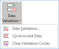
When you select the Data Validation option, a dialogue box appears. Within the dialogue box there are three options:
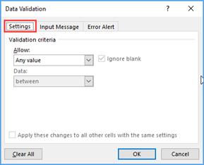
- Settings – This is where you’ll create the structure to control the data.
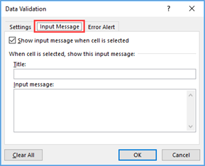
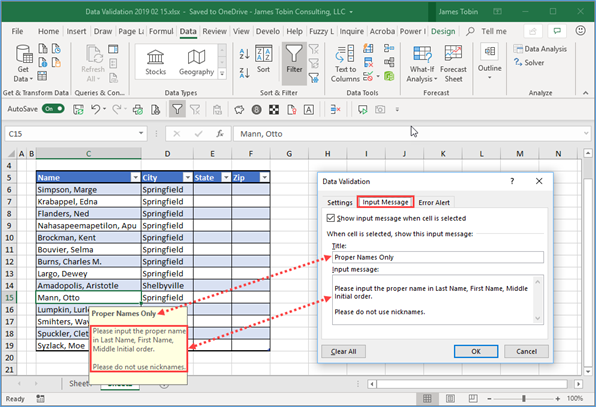
- Input Message – This tab is optional. You can create a custom message that will appear when the user selects a cell for data input. The Input Message and the Settings are not linked.
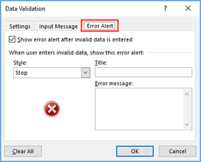
- Error Alert – This tab is optional. If you create a control in the Settings tab and you attempt to input incorrect data, Excel has a default error alert that will appear and let the user know the data is incorrect. However, you can create a custom error alert as you deem appropriate. The Error Alert and the Settings are not linked.
Settings
In the Settings tab, you’re given the option to set the validation criteria by category from the “Allow:” field. Refer to the table below for a brief description of the Categories. Generally speaking, the Data Validation categories allow you to restrict the type of data that is input into your tables.
| Category |
What the Category Means: |
| Any Value | This is the Excel’s default setting. There are no restrictions for these cells, and you can put anything you desire into the cell. |
| Whole Number | Only whole numbers (no decimals) are allowed for these cells. Choose limits or a range of numbers that can be entered. |
| Decimal | Only decimals (no whole numbers) are allowed for these cells. Choose limits or a range that can be entered. |
| List | This allows you to select the cell’s content from a dropdown list of your own creation. The list could be:
|
| Date | Only date values can be entered. You can limit the date or choose a range of allowable dates. |
| Time | Only time values can be entered. You can limit or choose a range of allowable dates and/or times.
Save Your Life Tip!! |
| Text Length | This ensures the text length is less than or equal to a specific number of characters. |
| Custom | This typically, requires a logic formula that will return a TRUE or FALSE. If the formula yields TRUE, the data is allowed, otherwise an error alert will appear. See examples below. |
The “Custom” category can be very powerful. I’ve included a few examples of logic formulae that I’ve used to ensure that the input meets the require criteria. Refer to the table below (Note that the “j5” reference refers to the first cell in an excel table that contains a custom data validation logic formula):
| Required Custom Criteria |
Formulae |
| Case – Lowercase Only | =exact(j5,lower(j5)) |
| Case – Uppercase Only | =exact(j5,upper(j5)) |
| No Duplicate Values | =countif($j$5:$j$17,j5)=1 |
| No Future Dates | =j5=today() |
| No Leading or Trailing Spaces | =j5=trim(j5) |
| No Numbers | =istext(j5) |
| No Text | =isnumber(j5) |
| No Weekends | =weekday(j5,2)<6 |
| Specific Leading Text | =exact(left(j5,4),”USA-“) |
| Text String Begins With… | =search(“t”,j5)=1 |
| Value in active cell is greater than the previous cell | =j6>j5 |
| Value in active cell keeps the column total below a budget cap | =sum($j$5:$J$17)<=10000 |
Input Message
The purpose of this section is to allow you to create a message that will be displayed when you select a cell that has a Data Validation Setting already assigned. For example, you can assign a title for the input message in the “Title:” bar and then place the instructions for the cell’s data in the “Input message:” box. When you click the OK button, the message will appear when you select a cell that has a Data Validation Setting already assigned. Note that the Settings and the Input message are not linked, so the setting assignment could end up being different that the input message.
Error Alert
As was mentioned above, Excel has a default error alert that will appear when the data input violates the structure established in the “Settings” tab. The default message appears as:

You’ll notice the “X” in the red circle in the default error alert. The “X” in the red circle means that the error alert is a “Stop” style error alert and will continue to appear until the correct data is input, or you remove the validation structure from the “Settings” tab. To continue inputting the correct data, hit “Retry”. Or, to stop inputting into the cell, hit “Cancel”.
There are three types of customizable error alert styles;
- Stop – This error alert has an “X” in the red circle on the left-hand side and requires that the correct information be input. Typically, this is my preferred error alert.
- Warning – This error alert has an “!” in a yellow triangle on the left-hand side and while providing a warning, you will be allowed to input bad data. With the “Warning” style, you are given a choice to continue with the bad data. If you select “No”, Excel will return you to the cell and allow you to input correct data. If you select “Yes”, the bad data will be placed in the cell.
- Information – This error alert has an “i” in a blue circle on the left-hand side and while perhaps imparting information, it will allow you to input bad data. When you hit OK, the bad data will be placed in the cell.
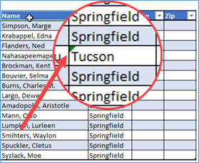
For the Warning and Information error alerts, should you accept the bad data, a green triangle will also be placed in the upper left-had corner of the cell containing the bad data, letting you know “something is rotten in the state of Denmark…”. The green triangle is a “help” for you to see the data that violates the structure in the “Settings” tab.
As mentioned, you can use Excel’s default “Stop” error alert or you can customize any of the three styles mentioned above. As examples:
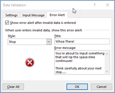
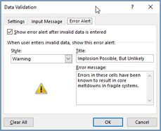
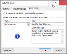
As invalid data is placed into cells, the error alerts appear. Error alerts corresponding to the examples above appear as:
|
Error Alert Style |
Custom Error Alert |
|
Stop |
 |
|
Warning |
 |
|
Information |
 |
Error Alerts are a great set of tools to help ensure that the data input meets your required standards.
Finding & Fixing Invalid Data
When you select the Data Validation feature from the Data ribbon, three options appear (see below). We’ve talked at length about the Data Validation but have not mentioned the circling/clearing of invalid data.


When you download data or allow invalid data to be input, Excel provides a quick way to identify the incorrect data.
After downloading data and applying the required criteria or after inputting bad data, select “Circle Invalid Data” from the Data Validation feature in the Data ribbon. When you do, the data that violates the criteria established in the Settings tab will be circled in red. For example:
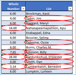
As you correct the individual datum, the red circle is removed.
If you’re ok with the data as presented, select “Clear Validation Circles” from the Data Validation feature in the Data ribbon. When you do, the data that violates the criteria established in the Settings tab will be unchanged, but the red circles will be gone.
Dependent Data Validation
There are times when you want to restrict the data choices based on previous valid data selections. This is known as Dependent Data Validation. This is a very powerful twist of the Data Validation feature.
As an example, you might have unique groups of products and within those unique groups, you might have unique groups of items. As you select a unique group of products, you then only want to see the unique items that correspond to that unique group. As an example, I’ve used this powerful twist in developing Budgets and Forecasts and in Materials Price Lists.
The key to accomplishing this is the List category within Data Validation. While using the List category, you’ll need to use Named Ranges and the Indirect function (=INDIRECT()).
As an example, below you’ll find a table of families with their corresponding members. As you select a family for the “Family” cell (E10), in the “Individual” cell (F10) you’ll want to be able to select one of the names of the individuals in that specific family.
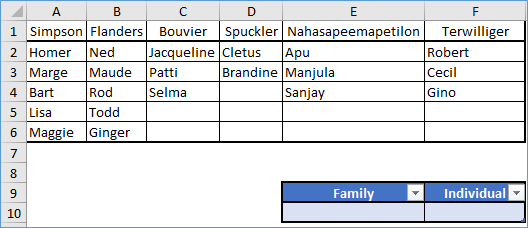
To begin, you’ll need to name the range that contains the family names (A1 through F1). Do to this, highlight A1 thru F1 and type Families in the name box (left of the formula bar), then hit Enter.
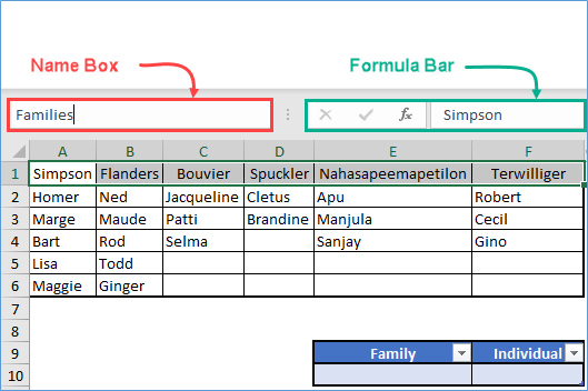
The range A1 through F1 is now named Families.
To create named ranges for each of the families, you’ll need to use the Ctrl key to highlight each family individually. For example:
- Highlight cells A1 through A6;
- Then while pressing and holding down the Ctrl key, highlight B1 through b6.
- Continue holding down the Ctrl key and highlight C1 through C4.
- Again, while holding down the Ctrl key, highlight D1 through D3.
- And again, while holding down the Ctrl key, highlight E1 through E4.
- And finally, while holding down the Ctrl key, highlight F1 through F4.
The highlighted areas should appear as:

All this precision highlighting and Ctrl key business may seem silly, but if you highlighted A1 through F6 and named the ranges, you’d get blank spaces for the families which contain less than 5 members. That’d be a bit sloppy, IMHO…
Please notice that between the vertical cell boundaries, there is a bit of white space on each side. This is Excel’s way of indicating that the highlighted sections are to be considered unique. If we selected A1 through F6 there’d be one solid mass of gray (highlighted area) with nothing unique.
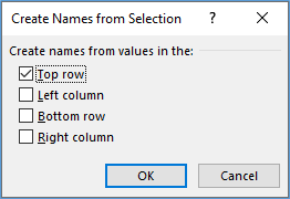
With the precision highlighting in place, press and hold the Ctrl + Shift + the F3 keys. This will open the “Create Names from Selection” dialogue box. Excel will “guess” by which values to name the ranges. However, you can select the correct one should Excel “guess” wrong. In this case, Excel guessed correctly and selected the top row to name the ranges. Hit OK to continue.
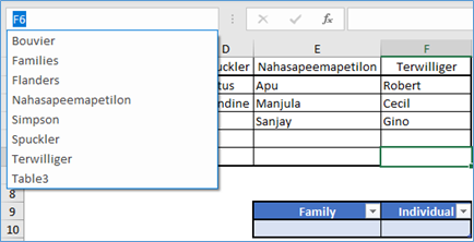
After hitting OK, Excel will name the precision highlighted areas using the name in the top row to create the unique named ranges. Click the dropdown button in the right-hand portion of the Name Box to see the newly created named ranges. You can see the new named ranges along with the previously name range “Families” (Table 3 refers to the 4 celled table in the lower right-hand side of the image.)
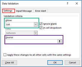
Now we need to assign the “Setting” in Data Validation. To begin, we need to assign a List in cell E10 to limit the selection of the families. Place the cell indicator (cursor) in cell E10. From the Data ribbon, select “Data Validation” and then “Data Validation…”. When the Data Validation dialogue box opens, from the Settings tab, select “List” from the “Allow:” field and move your cursor to the “Source:” field.
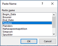
While in the “Source:” field, if you remember/know the named range you want to use, type the equals symbol (“=”) followed by the named range. If you need help remembering (and I almost always do…), with your cursor in the “Source:” field, press the F3 key and a dialogue box will appear allowing you to select a named range to use as the source for the list. Select the named range you desire, in this case “Families” and hit OK to continue.
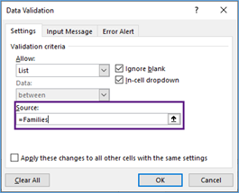
When you hit OK, Excel places the equals symbol (“=”) followed by the named range you selected into the “Source:” field. Hit OK to continue.
Place your cell indicator (cursor) in cell E10. As a result of the List requirement, a dropdown button appears and provides a list of valid names to choose from.
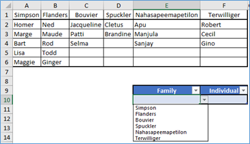
Once selected, move your cell indicator (cursor) in cell F10 (the Individual field).
Again, we need to assign the “Setting” in Data Validation for F10. To begin, we need to assign a List in cell F10 control the presentation of individual members of each of the families. Place the cell indicator (cursor) in cell E10. From the Data ribbon, select “Data Validation” and then “Data Validation…”. When the Data Validation dialogue box opens, from the Settings tab, select “List” from the “Allow:” field and move your cursor to the “Source:” field.
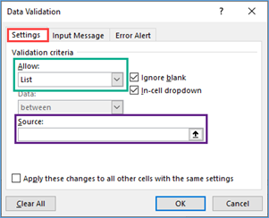
Here is where is gets a bit trickier (the twist!). You would think that you could refer to E10 and Excel would call up the corresponding named range, but it won’t. It will only recognize the contents of E10 as text. To trick Excel into treating the contents of cell E10 (Family) as a named variable, you need to use the Indirect function (=INDIRECT()) in the “Source:” field as follows:
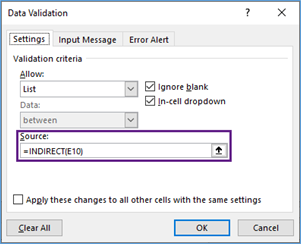
In this case, the Indirect function takes the resulting text string in E10 and converts it to a valid reference. As a result, only the names of a specific family are listed as dependent on the contents of E10 (Family).
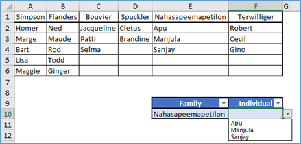
Please note that if you change the family in E10, the individual will not change (and may remain wrong), until you change it.

Leave a Reply